Solving Lane-Emden via Shooting#
We’ll use 4th order RK integration and we’ll integrate both inward from the surface and outward from the center and meet at some point in the middle, \(\xi_\mathrm{fit}\).
As before, our system is:
with the limit near \(\xi \rightarrow 0\) of
We’re going to integrate outward from the center and inward from the surface and meet in the middle.
At the center, our boundary conditions are:
\(y(0) = 1\)
\(z(0) = 0\)
and at the surface, \(\xi_s\), they are:
\(y(\xi_s) = 0\)
\(z(\xi_s) = \eta\)
Initially, we don’t know either \(\eta\) or \(\xi_s\).
Our algorithm will proceed as follows:
Take an initial guess for \(\eta\) and \(\xi_s\). Pick \(\xi_f = \xi_s/2\).
Integrate from the center outward to the fit point, \(\xi_f\), getting the solution: \(y_\mathrm{out}(\xi_f)\), \(z_\mathrm{out}(\xi_f)\).
Integrate from the surface (starting at the guess \(\xi_s\)) inward to the fit point, getting the solution \(y_\mathrm{in}(\xi_f)\), \(z_\mathrm{in}(\xi_f)\)
Constrain the solution to match at the fit point by finding the zero of:
\[\begin{align*} Y(\eta, \xi_s) &\equiv y_\mathrm{in}(\xi_f) - y_\mathrm{out}(\xi_f) = 0 \\ Z(\eta, \xi_s) &\equiv z_\mathrm{in}(\xi_f) - z_\mathrm{out}(\xi_f) = 0 \end{align*}\]we will do this via the secant method. This will yield a new guess for \(\eta\) and \(\xi_s\).
Iterate over this procedure until the \(\eta\) and \(\xi_s\) converge.
import numpy as np
import matplotlib.pyplot as plt
from scipy.integrate import solve_ivp
def rhs(xi, H, n):

    y = H[0]
    z = H[1]

    f0 = z

    if xi == 0.0:
        f1 = 2.0/3.0 - y**n
    else:
        f1 = -2.0*z/xi - y**n

    return np.array([f0, f1])
We’ll use SciPy’s implementation of 4th order Runge-Kutta here
def le_integrate(xi_start, xi_end, H0, n):

    sol = solve_ivp(rhs, (xi_start, xi_end), H0,
                    method="RK45", rtol=1.e-8, atol=1.e-8, args=(n,))

    xi = sol.t
    y = sol.y[0, :]
    z = sol.y[1, :]

    return xi, y, z
We need to find the roots of our system that matches the solution at the midpoint.
Let’s Taylor expand our functions \(Y\) and \(Z\):
We want to solve for the corrections, \(\Delta \eta\) and \(\Delta \xi_s\) that zero this—this is Newton’s method, but now for a system of equations.
We can solve the first equation for \(\Delta \eta\):
and then substitute this into the second equation and solve for \(\Delta \xi_s\):
We still need the derivatives, which we will compute via differencing.
def solve_le(n):

    # initial guesses for the unknowns -- if we aren't careful with the
    # guess at the outer boundary, we can get 2 roots.  Here we know that
    # n = 1 has xi_s = pi

    if n > 2.0:
        xi_s = 8.0
    else:
        xi_s = np.pi

    eta = -0.01

    # for numerical differentiation
    eps = 1.e-8

    # main iteration loop
    converged = False
    while not converged:

        # fitting point
        xi_fit = xi_s / 2.0

        # baseline integration

        # outward from the center
        xi_out, y_out, z_out = le_integrate(0.0, xi_fit, [1.0, 0.0], n)

        # inward from xi_s
        xi_in, y_in, z_in = le_integrate(xi_s, xi_fit, [0.0, eta], n)

        # the two functions we want to zero
        Ybase = y_in[-1] - y_out[-1]
        Zbase = z_in[-1] - z_out[-1]

        # now do eta + eps*eta, xi_s
        # inward from xi_s
        H0 = np.array([0.0, eta*(1.0+eps)])
        xi_in, y_in, z_in = le_integrate(xi_s, xi_fit, [0.0, eta * (1.0 + eps)], n)

        Ya = y_in[-1] - y_out[-1]
        Za = z_in[-1] - z_out[-1]

        # our derivatives
        dYdeta = (Ya - Ybase) / (eta * eps)
        dZdeta = (Za - Zbase) / (eta * eps)

        # now do alpha, xi_s + eps*xi_s
        # inward from xi_s
        xi_in, y_in, z_in = le_integrate(xi_s  * (1.0 + eps), xi_fit, [0.0, eta], n)

        Yxi = y_in[-1] - y_out[-1]
        Zxi = z_in[-1] - z_out[-1]

        # our derivatives
        dYdxi_s = (Yxi - Ybase) / (xi_s * eps)
        dZdxi_s = (Zxi - Zbase) / (xi_s * eps)

        # compute the correction for our two parameters
        dxi_s = - (Zbase - dZdeta * Ybase / dYdeta) / \
                    (dZdxi_s - dZdeta * dYdxi_s / dYdeta)

        deta = -(Ybase + dYdxi_s * dxi_s) / dYdeta

        # limit the changes per iteration
        deta = min(abs(deta), 0.1 * abs(eta)) * np.copysign(1.0, deta)
        dxi_s = min(abs(dxi_s), 0.1 * abs(xi_s)) * np.copysign(1.0, dxi_s)

        print(f"corrections:  {deta:13.10f}, {dxi_s:13.10f}")

        eta += deta
        xi_s += dxi_s

        if abs(deta) < eps * abs(eta) and abs(dxi_s) < eps * abs(xi_s):
            converged = True

    return xi_in, y_in, z_in, xi_out, y_out, z_out
n = 3
xi_in, y_in, z_in, xi_out, y_out, z_out = solve_le(n)
corrections:  -0.0010000000, -0.8000000000
corrections:  -0.0011000000,  0.1041147613
corrections:  -0.0012100000, -0.4023129572
corrections:  -0.0013310000,  0.6901801804
corrections:  -0.0014641000, -0.7591981985
corrections:  -0.0016105100,  0.6832783786
corrections:  -0.0017715610, -0.7516062165
corrections:  -0.0019487171,  0.6764455948
corrections:  -0.0021435888, -0.7440901543
corrections:  -0.0023579477,  0.6696811389
corrections:  -0.0025937425, -0.6416950043
corrections:  -0.0028531167,  0.5277799831
corrections:  -0.0031384284, -0.4366093478
corrections:  -0.0034522712,  0.1755125576
corrections:  -0.0037974983, -0.0987624438
corrections:  -0.0006486268,  0.0046186327
corrections:  -0.0000086425, -0.0004880733
corrections:  -0.0000000003,  0.0000000612
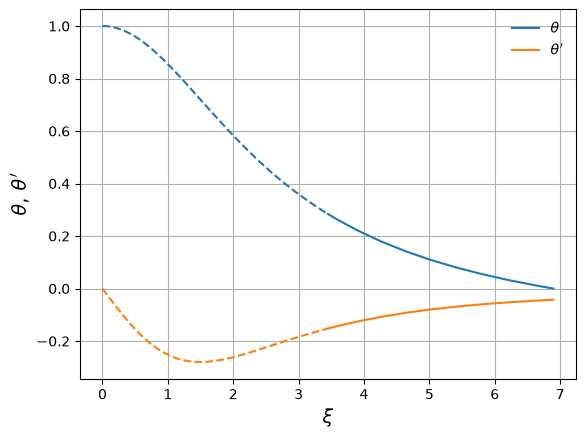
fig, ax = plt.subplots()

ax.plot(xi_in, y_in, color="C0", label=r"$\theta$")
ax.plot(xi_out, y_out, color="C0", ls="--")

ax.plot(xi_in, z_in, color="C1", label=r"$\theta'$")
ax.plot(xi_out, z_out, color="C1", ls="--")

ax.set_xlabel(r"$\xi$", fontsize=14)
ax.set_ylabel(r"$\theta,\, \theta'$", fontsize=14)

ax.legend(frameon=False, loc="best")
ax.grid()
Now we can get the surface of the polytrope, \(\xi_1\)
xi1 = xi_in[0]
xi1
np.float64(6.896848900813273)
and \(\theta^\prime\) at the surface:
dthetadxi_1 = z_in[0]
A common quantity needed in finding physical values is \(-\xi_1^2 \theta^\prime |_{\xi=\xi_1}\)
-xi1**2 * dthetadxi_1
np.float64(2.0182358018117537)