Convective temperature gradient

Let’s visualize what a convectively-unstable temperature gradient looks like. We’ll create two plane-parallel atmospheres: one isothermal (stable against convection) and one isentropic (convectively-unstable).

For plane-parallel, we can take the gravitational acceleration, \(g\), as constant, and write hydrostatic equilibrium as:

\[\frac{dP}{dr} = -\rho |g|\]

Isothermal

For an isothermal atmosphere, and assuming an ideal gas, we can take:

\[P = \frac{\rho k_B T}{\mu m_u}\]

and inserting this into HSE, we have:

\[\frac{k_B T}{\mu m_u} \frac{d\rho}{dr} = -\rho |g|\]

(where we used the fact that \(T\) is constant to pull it out of the derivative. Then rewriting:

\[\frac{d\rho}{\rho} = - \frac{\mu m_u |g|}{k_B T} = - \frac{dr}{H}\]

where \(H\) is the pressure scale height:

\[H^{-1} = \frac{1}{P} \left | \frac{dP}{dr} \right | = \frac{\rho |g|}{P} = \frac{\mu m_u |g|}{k_B T}\]

This can be easily integrated to give:

\[\rho(r) = \rho_0 e^{-r/H}\]

and in terms of pressure,

\[P(r) = P_0 e^{-r/H}\]

Isentropic

If the atmosphere has constant entropy, we can use the adiabatic relation between pressure and density:

\[P = K \rho^{\gamma}\]

Putting this in HSE, we have:

\[\begin{align*} \gamma K \rho^{\gamma - 1} \frac{d\rho}{dr} &= -\rho |g| \\ \rho^{\gamma - 2} d\rho &= - \frac{|g|}{\gamma K} dr \end{align*}\]

Density

This can be integrated. We take \(P(r = 0) = P_0\), \(\rho(r=0) = \rho_0\) and find:

\[\rho(r) = \rho_0 \left ( 1 - \frac{\gamma - 1}{\gamma} \frac{|g|}{K} \frac{1}{\rho_0^{\gamma - 1}} r \right )^{1/(\gamma - 1)}\]

we can eliminate \(K\) as \(K = P_0 / \rho_0^{\gamma}\) and get:

\[\rho(r) = \rho_0 \left ( 1 - \frac{\gamma - 1}{\gamma} \frac{|g|\rho_0}{P_0} r \right )^{1/(\gamma - 1)}\]

or in terms of the scale height, \(H = P_0 / (\rho_0 |g|)\),

\[\rho(r) = \rho_0 \left ( 1 - \frac{\gamma - 1}{\gamma} \frac{r}{H} \right )^{1/(\gamma - 1)}\]

Pressure

Since \(P(r) = K\rho^{\gamma}\), we have:

\[P(r) = P_0 \left ( 1 - \frac{\gamma - 1}{\gamma} \frac{r}{H} \right )^{\gamma/(\gamma - 1)}\]

Temperature

Finally, if we assume an ideal gas, then

\[T = \frac{\mu m_u}{k_B}\frac{P}{\rho} = T_0 \left (1 - \frac{\gamma - 1}{\gamma} \frac{r}{H} \right )\]

where \(T_0 = \mu m_u P_0 / (k_B \rho_0)\).

The temperature just falls off linearly (for an ideal gas).

Note

If we differentiate this temperature profile, we get:

\[\frac{dT}{dr} = \frac{T_0}{H} \left (1 - \frac{1}{\gamma} \right )\]

This is just the adiabatic temperature gradient, \(dT/dr |_\mathrm{ad}\)!

Comparisons

We can plot these thermodynamic profiles as a function of \(\xi \equiv r/H\)

import matplotlib.pyplot as plt
import numpy as np

xi = np.linspace(0, 5, 100)

gamma = 5./3.

P_isothermal = np.exp(-xi)

P_isentropic = (1 - (gamma - 1)/gamma * xi)**(gamma/(gamma-1))

/tmp/ipykernel_2449/2183992313.py:5: RuntimeWarning: invalid value encountered in power
  P_isentropic = (1 - (gamma - 1)/gamma * xi)**(gamma/(gamma-1))

fig, ax = plt.subplots()

ax.plot(xi, P_isothermal, label="isothermal")
ax.plot(xi, P_isentropic, label="isentropic")

ax.set_xlabel("$r/H$")
ax.set_ylabel("$P/P_0$")

ax.legend()
ax.grid(linestyle=":")

fig.savefig("atm.png")

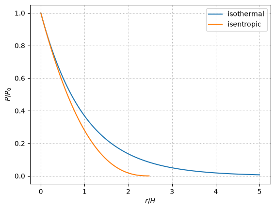
For the same base pressure, the isothermal atmosphere is more extended than the isentropic one.