Measuring Convergence of our Euler Solver#

We measured convergence with advection by comparing to the exact solution. But what about the case when we don’t know the exact solution? We can use a grid convergence study to assess the convergence. Here’s how it works.

1. Pick a smooth problem – a good problem is the acoustic pulse described in this paper:

   A high-order finite-volume method for conservation laws on locally refined grids

   See section 4.2. You’ll do this in 1-d in our solver with periodic BCs.

2. Run the problem at 4 different resolutions, each varying by a factor of 2, e.g., 32, 64, 128, and 256 zones.

3. Compute an error between the run with N zones and the run with 2N zones as follows:

   • Coarsen the problem with 2N zones down to N zones by averaging 2 fine zones into a single coarse zone. This is shown below:

     

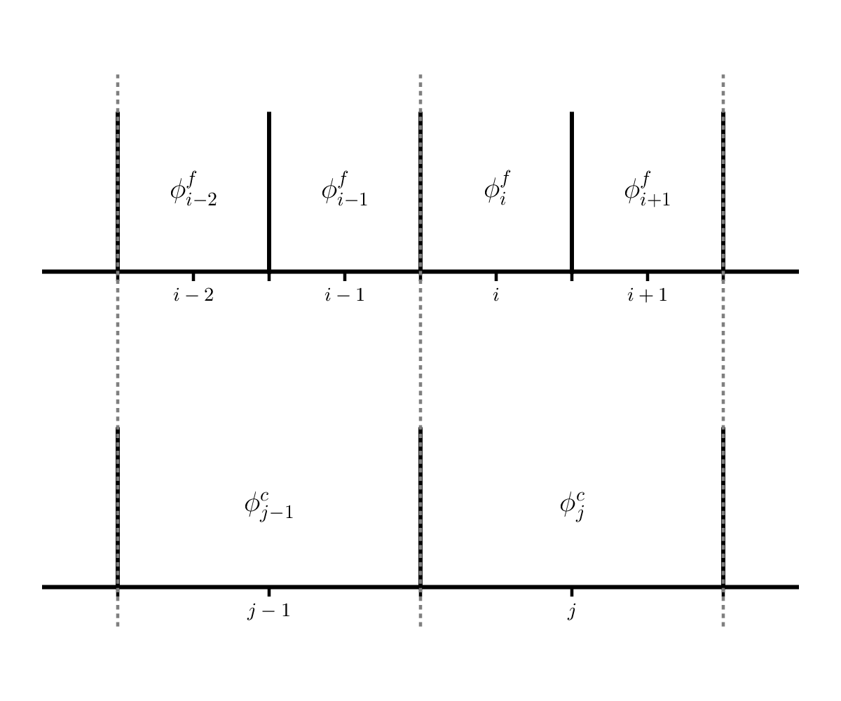
     Here, ${\varphi }^f$ is a variable on the finer resolution grid and ${\varphi }^c$ is the variable on the coarse grid. We see that ${\varphi }_j^c$ has two fine grid counterparts: ${\varphi }_i^f$ and ${\varphi }_{i+1}^f$, so we would do:

     $${\varphi }_j^c=\frac{1}{2}({\varphi }_i^f+{\varphi }_{i+1}^f)$$

   • Compute the $L_2$-norm of the difference between the coarsened 2N zone run and the N zone run.

   • Do this for all pairs, so for the 4 runs proposed above, you’d have 3 errors corresponding to 64-128, 128-256, and 256-512.

4. Plot the errors along with a line representing ideal 2nd order convergence.