Measuring Convergence

In order to see whether our methods are working as designed, we need to be able to measure the convergence rate.
We have \(N\) points in our solution, so we need to define a metric that allows us to quantify the error.

We’ll define a vector norm, the \(L_2\) norm, for a set of discrete data \(\phi_i\), as:

\[\|\phi\|_2 = \left ( \Delta x \sum_{i=0}^{N-1} \phi_i^2 \right )^{1/2}\]

and then we can define an error as \(e_i = a_i - a^\mathrm{exact}(x_i)\) for all the points in our domain and compute an error, \(\epsilon\) as \(\| e\|_2\). Further, for our problem, after 1 period, we know that the exact solution is just the initial data, so we can write:

\[\epsilon = \| a_i^\mathrm{final} - a_i^\mathrm{initial} \|_2 = \left [ \Delta x \sum_{i=0}^{N-1} (a_i^\mathrm{final} - a_i^\mathrm{initial} )^2 \right ]^{1/2}\]

Note

It only makes sense to discuss convergence if the initial conditions themselves converge. For the top hat, there is a discontinuity, and as we increase and increase the resolution, we will never resolve the step. So the top hat is not a good set of initial conditions to assess convergence. We should use a smooth problem.

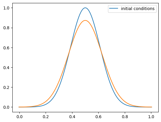
We’ll look at the Gaussian.

Our solver and the initial conditions are available in a module, advection

import advection

And here are our initial conditions

def sine(g):
    g.a[:] = 1.0 + 0.5 * np.sin(2.0*np.pi*g.x)

C = 0.5
u = 1.0
nx = 128

g = advection.advection(nx, u, C, init_cond=advection.gaussian)
fig = g.plot()

Our FVGrid class has a method to compute the norm

import inspect
print(inspect.getsource(g.norm))

    def norm(self, e):
        """ return the norm of quantity e which lives on the grid """
        if not len(e) == (2*self.ng + self.nx):
            return None

        return np.sqrt(self.dx*np.sum(e[self.ilo:self.ihi+1]**2))

Let’s try this out

u = 1.0
C = 0.5

for nx in [32, 64, 128, 256, 512]:
    g = advection.advection(nx, u, C, init_cond=advection.gaussian)
    print(f"{nx:3d} {g.norm(g.a - g.ainit):7.4f}")

 32  0.1396
 64  0.0877
128  0.0506
256  0.0275
512  0.0144

As we see, this is demonstrating first-order convergence—as we double the number of cells, the error is decreasing by a almost a factor of 2.

Exercise

Try running the convergence test with the top hat initial conditions