Implementing First Order Advection#
We now have all the pieces needed to implement first-order accurate advection.
import numpy as np
import matplotlib.pyplot as plt
For convenience, the grid module can be downloaded as a file fv_grid.py and placed in the same directory as this notebook. Then it can be imported
import fv_grid
Now we’ll write our driver. We’ll take as input:
nx: the number of zonesu: the advective velocityC: the CFL number
we can also specify the number of periods and pass in the function that supplies the initial conditions
def advection(nx, u, C, num_periods=1, init_cond=None):

    # create the grid
    g = fv_grid.FVGrid(nx, ng=1)

    # compute the stop time
    t_period = (g.xmax - g.xmin) / np.abs(u)
    tmax = num_periods * t_period

    # setup the initial conditions and store them for later
    # plotting
    init_cond(g)
    g.ainit[:] = g.a[:]

    # compute the timestep
    dt = C * g.dx / np.abs(u)

    # evolution loop
    t = 0.0
    while t < tmax:
        if t + dt > tmax:
            dt = tmax - t

        g.fill_BCs(g.a)

        # get the interface states -- just piecewise constant -- we need
        # an interface state on each boundary, so for nx zones there are
        # nx + 1 interface states

        aleft = g.scratch_array()
        aleft[g.ilo:g.ihi+2] = g.a[g.ilo-1:g.ihi+1]

        aright = g.scratch_array()
        aright[g.ilo:g.ihi+2] = g.a[g.ilo:g.ihi+2]

        # solve the Riemann problem -- just upwinding
        aint = np.where(u > 0, aleft, aright)

        # compute the fluxes
        flux = u * aint

        # conservative update
        g.a[g.ilo:g.ihi+1] += -dt/g.dx * (flux[g.ilo+1:g.ihi+2] - flux[g.ilo:g.ihi+1])

        t += dt

    return g
Initial conditions#
We need to supply a function that provides the initial conditions. It has the signature:
init_cond(FVGrid)
First up: the tophat
def tophat(g):
    g.a[:] = 0.0
    g.a[np.logical_and(g.x >= 1./3, g.x <= 2./3.)] = 1.0
Now we’ll run it.
nx = 128
u = 1
C = 0.8
g = advection(nx, u, C, init_cond=tophat)
fig = g.plot()
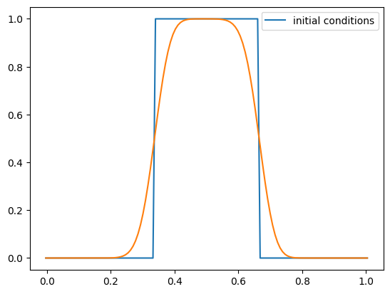
This is very diffusive, but that’s to be expected for a first-order accurate method.
Now let’s try the Gaussian initial conditions
def gaussian(g):
    g.a[:] = np.exp(-40.0*(g.x - 0.5)**2)
g = advection(nx, u, C, init_cond=gaussian)
fig = g.plot()
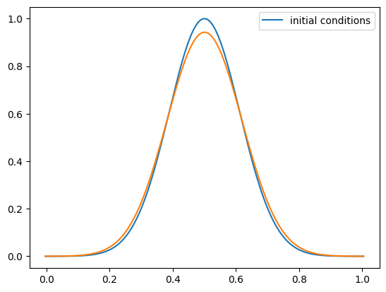
This looks a little better—we can still see the basic shape.