Equilibrium

At high temperatures, the reverse rates become important and we can come into equilibrium—resulting in nuclear statistical equilibrium (NSE).

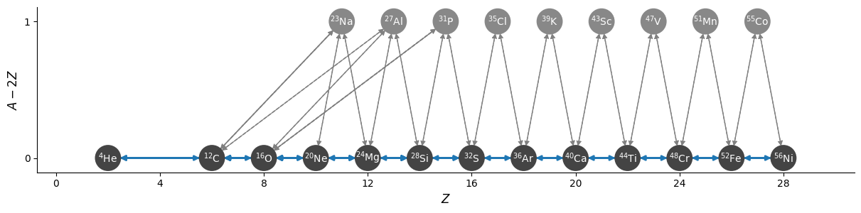
Let’s see this by reintegrating our “aprox13” network.

import pynucastro as pyna

net = pyna.network_helper(["p", "he4",
                           "c12", "o16", "ne20", "na23",
                           "mg24", "al27", "si28", "p31", "s32",
                           "cl35", "ar36", "k39", "ca40",
                           "sc43", "ti44", "v47", "cr48",
                           "mn51", "fe52", "co55", "ni56"])

from pynucastro.rates.aprox_family_rates import make_CO_approx_rates

approx_net = pyna.PythonNetwork(rates=net.get_rates())

approx_net.make_CO_burning_approx("C")
approx_net.remove_nuclei(["na23"])

approx_net.make_CO_burning_approx("CO")
approx_net.remove_nuclei(["al27"])

approx_net.make_CO_burning_approx("O")
approx_net.remove_nuclei(["p31"])

approx_net.make_ap_pg_approx(intermediate_nuclei=["cl35", "k39", "sc43", "v47", "mn51", "co55"])
approx_net.remove_nuclei(["cl35", "k39", "sc43", "v47", "mn51", "co55"])

fig = approx_net.plot(rotated=True,
                      size=(1200, 300), node_size=600, node_font_size=10)

Now let’s pick a very high temperature.

rho = 1.e7
T = 6.e9

comp = pyna.Composition(approx_net.unique_nuclei, small=0.0)
comp.X[pyna.Nucleus("he4")] = 1.0
Y0 = comp.get_molar_array()

tmax = 100.0

sol_approx = approx_net.integrate_network(tmax, rho, T, Y0, rtol=1.e-6)

/opt/hostedtoolcache/Python/3.14.5/x64/lib/python3.14/site-packages/pynucastro/rates/derived_rate.py:125: UserWarning: C12 partition function is not supported by tables: set log_pf = 0.0 by default
  warnings.warn(UserWarning(f'{nuc} partition function is not supported by tables: set log_pf = 0.0 by default'))

fig = sol_approx.plot_evolution(three_level_style=True, ymin=1.e-8)

/opt/hostedtoolcache/Python/3.14.5/x64/lib/python3.14/site-packages/pynucastro/networks/python_network.py:412: UserWarning: Attempt to set non-positive xlim on a log-scaled axis will be ignored.
  ax.set_xlim(tmin, tmax)

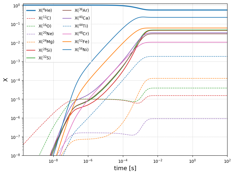
Now we see that after about \(10^{-2}~\mathrm{s}\), we enter equilibrium (\(dX/dt = 0\)).

NSE

We can solve for nuclear statistic equilibrium directly. Here’s an overview (taken from pynucastro’s intro to NSE

NSE assumptions

To get the NSE constraint equations we assume:

• every isotope is connected to the free nucleons, neutrons and protons, through a series of strong nuclear reactions.

• we are in chemical equilibrium, so

  \[(A, Z) \rightleftharpoons Z \ \mathrm{p} + N \ \mathrm{n}\]

  giving:

  \[\mu_i = Z_i \mu_p + N_i \mu_n\]

• The nuclei obey Maxwell-Boltzmann statistics, so:

  \[\mu_i = \mu_i^{\mathrm{kin}} + m_i c^2 + \mu_i^c\]

  where \(\mu_i^c\) is the Coulomb potential and

  \[\mu_i^{\mathrm{kin}} = Z_i (\mu_p^{\mathrm{kin}} + \mu_p^c) + N_i \mu_n^{\mathrm{kin}} + \underbrace{(Z_i m_p + N_i m_n - m_i) c^2}_{B_i} - \mu^c_i\]

  where \(B_i\) is the binding energy of the isotope.

  Maxwell-Boltzmann statistics then give us:

  \[X_{i, \mathrm{NSE}} = \dfrac{(m_i)^{5/2}}{\rho} g_i \left( \dfrac{k_B T}{2\pi \hbar^2} \right)^{3 /2} \exp{\left( \dfrac{Z_i (\mu_p^{\mathrm{kin}} + \mu_p^c) + N_i \mu_n^{\mathrm{kin}} + B_i - \mu^c _i}{k_B T} \right)}\]

NSE constraint equations

NSE allows us to just solve for \(\mu_p^{\mathrm{kin}}\) and \(\mu_n^{\mathrm{kin}}\) via:

• Conservation of mass:

  \[\sum_i X_i^{\mathrm{NSE}}(\mu_p^{\mathrm{kin}}, \mu_n^{\mathrm{kin}}) - 1 = 0\]

• Conservation of charge:

  \[\sum_i \frac{Z_i}{A_i} X_i^{\mathrm{NSE}} (\mu_p^{\mathrm{kin}}, \mu_n^{\mathrm{kin}}) - Y_e = 0\]

We can create a network that knows about NSE

nse_net = pyna.NSENetwork(rates=approx_net.get_rates())

Now we can solve for the NSE state. The only composition information we need to provide is the electron fraction.

comp_nse = nse_net.get_comp_nse(rho, T, comp.ye)

fig = comp_nse.plot()

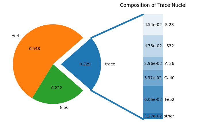
If we are in equilibrium, then no integration is needed.