Lab model revisited

Let’s reload the profiles our lab with the Na23-Ne23 rates and see what they say about the Fermi energy.

import mesa_reader as mr
import numpy as np

model1 = mr.MesaData("lab1/profile1.data")
model2 = mr.MesaData("lab1/profile2.data")

r1 = 10.0**model1.logR
m1 = model1.mass
rho1 = 10.0**model1.logRho
T1 = 10.0**model1.logT

r2 = 10.0**model2.logR
m2 = model2.mass
rho2 = 10.0**model2.logRho
T2 = 10.0**model2.logT

Finding the Fermi energy in our model

We can compute the Fermi energy, by getting the degeneracy parameter:

\[\eta = \mathcal{E}_F/(kT) = (\mu - m_e c^2)/(kT)\]

So

\[\mathcal{E}_F = \eta k T\]

Note that this is the kinetic energy, since the rest mass was subtracted off. This is the energy that is available to overcome the energy difference in nuclei and electron-capture.

We can compute the Fermi energy from the Fermi-Dirac distribution:

\[n_e = \frac{\rho Y_e}{m_u} = \frac{8\pi}{h^3} \int_0^\infty \frac{p^2}{e^{\mathcal{E}(p)/k_B T - \eta} + 1} dp\]

with

\[\mathcal{E}(p) = m_e c^2 \left [ \sqrt{1 + \left ( \frac{p}{m_e c} \right )^2 } - 1 \right ]\]

Given the density and \(Y_e\), we can root-find on this to get \(\eta\)

import pynucastro as pyna
from pynucastro import mesa_utils

eos = pyna.eos.ElectronEOS()

kB = pyna.constants.constants.k
erg2MeV = pyna.constants.constants.erg2MeV

We’ll work with the late time model

mesa_zones = mesa_utils.get_all_data(model2)

Note: this is slow cause it’s doing the integration directly.

E_fermi = np.zeros_like(rho2)
for i, v in mesa_zones.items():
    rho, T, comp = v
    es, ps = eos.pe_state(rho, T, comp, compute_derivs=False)
    eta = es.eta
    E_fermi[i] = eta * kB * T

E_fermi *= erg2MeV

import matplotlib.pyplot as plt

fig, ax = plt.subplots()
ax.semilogx(r2, E_fermi)
ax.set_xlabel(r"radius ($R_\odot$)")
ax.set_ylabel(r"$\mathcal{E}_\mathrm{Fermi}$ (MeV)")
ax.grid(ls=":")

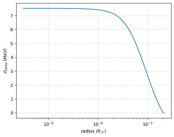
Notice that the Fermi energy is highest at the core of the WD, as expected. And it is > 7 MeV, which is large comparable to the typical binding energy / nucleon in a nucleus.

Correspondence with Urca shell

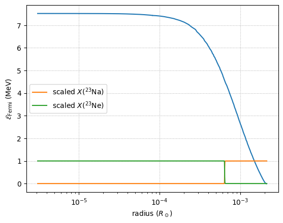
Let’s overlay \(X({}^{23}\mathrm{Na})\) and \(X({}^{23}\mathrm{Ne})\). Their mass-fractions are small, so we’ll scale by the maximum to make them \(\mathcal{O}(1)\) in the plot.

X_na23 = model2.na23
X_ne23 = model2.ne23
scale = max(X_na23.max(), X_ne23.max())

ax.semilogx(r2, X_na23/scale, label=r"scaled $X({}^{23}\mathrm{Na})$")
ax.semilogx(r2, X_ne23/scale, label=r"scaled $X({}^{23}\mathrm{Ne})$")
ax.legend()
fig

Now let’s compute the Q-value of the reaction to figure out what Fermi energy should be the threshold

Na23 = pyna.Nucleus("na23")
Ne23 = pyna.Nucleus("ne23")
Q = Ne23.mass - Na23.mass
Q

4.375803499999165

Note that these are the atomic masses, from Nubase, so they include the electron mass (we’ll neglect the atomic binding energy)

E_thresh = Q

Now, where is this in our model?

idx = np.where(E_fermi > E_thresh)[0][0]
idx

np.int64(373)

we’ll draw a vertical line indicating where \(\mathcal{E}_\mathrm{Fermi} \sim Q\)

ax.axvline(r2[idx], color="0.25", ls="--")
ax.text(r2[idx], 4, r"radius where $\mathcal{E}_\mathrm{Fermi} \sim Q$",
        rotation=270, color="0.25", verticalalignment="center")
fig

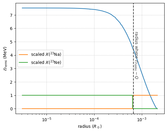
Notice that the location of \(\mathcal{E}_\mathrm{Fermi} = Q\) corresponds to the radius where the \(A=23\) Urca pair nuclei switch abundances.

Important

This is approximate, since we are ignoring the structure of the nuclei and its energy levels.