EOS regimes

Recall, we’ll consider:

• ions (assume full ionization)

• electrons

• radiation

We can look at the \(\rho\)-\(T\) plane to understand where each of the components of the EOS dominate.

import numpy as np
import matplotlib.pyplot as plt

Physical constants, all in CGS

m_e = 9.11e-28
m_u = 1.66e-24
c = 3.e10
k = 1.38e-16
h = 6.63e-27
a = 5.67e-15
e = 4.8e-10 # esu

Some composition info. We’ll specify

• mean molecular weight per electron:

  \[\mu_e = \left [ \sum_k \frac{Z_k X_k}{A_k} \right ]^{-1}\]

  we often work with electron fraction, \(Y_e = 1/\mu_e\)

• mean molecular weight of the ions:

  \[\mu_I = \left [ \sum_k \frac{X_k}{A_k} \right ]^{-1}\]

• total mean molecular weight:

  \[\frac{1}{\mu} = \frac{1}{\mu_e} + \frac{1}{\mu_I}\]

mu_e = 2
mu_I = 12.0

mu = 1.0 / (1.0/mu_e + 1.0/mu_I)

# for crystallization, we need the charge of the ions
Z = 6.0

Degeneracy vs. Ideal gas

We find the (dimensionless) Fermi momentum (\(x_F = p_F / (mc)\)) via

\[n_e = \frac{\rho}{\mu_e m_u} = \int_0^{x_F} x^2 dx\]

where we assume complete degeneracy (so the distribution function is just a step-function). This gives

\[x_F = \left ( \frac{\rho}{\mu_e B} \right )^{1/3}\]

where the constant \(B\) is:

\[B = \frac{8\pi}{3} m_u \left (\frac{m_e c}{h} \right )^3\]

We then define the transition to degeracy by comparing to the thermal energy, \(k T\)

\[\mathcal{E}_F = m_e c^2 \left ( \sqrt{1 + x_F^2} - 1 \right ) \sim k T\]

Here’s a function that computes this line

# Fermi momentum constant (from number density integral)
B = (8.0*np.pi/3.0)*m_u*(m_e*c/h)**3

def deg_ideal(rho, mu_e=2.0):
    """temperature on the line separating degeneracy and ideal gas as a function
 of rho"""

    # dimensionless Fermi momentum
    x_F = (rho / mu_e / B)**(1./3.)

    # set E_F = k T
    T = (1./k) * m_e * c**2 * (np.sqrt(1 + x_F**2) - 1)

    return T

Ideal gas vs. radiation

A simple way to determine whether an ideal case or radiation dominates is to set their energy densities equal. At the temperatures where we expect this to occur, we will assume that the electrons are not degenerate, so we will use the full \(\mu\) for the composition in the ideal gas instead of \(\mu_I\).

Our line is:

\[\frac{\rho k T}{\mu m_u} \sim \frac{1}{3}a T^4\]

Here’s a function that computes this

def rad_ideal(rho, mu=0.5):
    """temperature on the line separating radiation and ideal gas as a function 
of rho"""

    T = ((3 * k / (m_u * a)) * (rho / mu))**(1./3.)
    return T

Crystallization

Finally, at low temperatures and high densities, the ions can crystallize. The comparison where is the thermal energy to the Coulomb energy:

\[\Gamma = \frac{kT}{Z^2 e^2 / a}\]

where we take \(\Gamma = 175\) as the point where crystallization sets in (see Equation of state of fully ionized electron-ion plasmas. II. Extension to relativistic densities and to the solid phase by Potekhin & Chabrier 2002).

The separation between ions, \(a\) is found via:

\[V = n_I^{-1} = \frac{\mu_I m_u}{\rho} = \frac{4\pi}{3} a^3\]

Putting this together, the expression for the boundary of crystallization is computed below

def crystallization(rho):
    """temperature where crystallization of ions sets in"""
    Gamma_C = 175
    
    T = ((rho / mu_I) * (Z**2 * e**2 / (Gamma_C * k))**3 * (4.0 * np.pi / 3.0 / 
m_u))**(1./3.)
    return T

Plotting the boundaries

rho = np.logspace(-5, 10, 2000)

fig = plt.figure()
ax = fig.add_subplot(111)

ax.plot(rho, deg_ideal(rho))
ax.plot(rho, rad_ideal(rho))
ax.plot(rho, crystallization(rho))

# NR vs ER degeneracy
ax.vlines(B*mu_e, 1.e4, 1.e10, color="0.5", ls=":")


ax.text(1.e-2, 1.e9, "radiation\ndominates", horizontalalignment="center")
ax.text(1.e-3, 1.e5, "ideal gas", horizontalalignment="center")
ax.text(1.e3, 1.e5, "NR electron\ndegeneracy", horizontalalignment="center")
ax.text(1.e9, 1.e8, "ER electron\ndegeneracy", horizontalalignment="center")
ax.text(1.e5, 1.e3, "crystallization", horizontalalignment="center")

ax.text(150, 1.5e7, "⊙")
ax.text(1.e6, 1.e7, r"$\times$"+"\nWD (low)", horizontalalignment="center", fontsize="small")
ax.text(2.e9, 1.e7, r"$\times$"+"\nWD (high)", horizontalalignment="center", fontsize="small")

ax.set_xscale("log")
ax.set_yscale("log")

ax.set_xlabel(r"$\rho$ (g/cc)")
ax.set_ylabel("$T$ (K)")
ax.grid(ls=":")

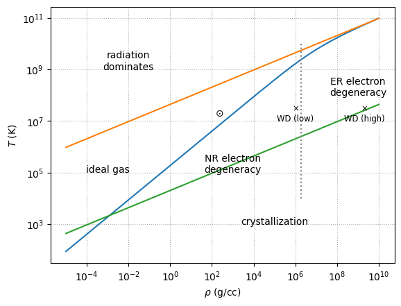
Some representative WD positions are marked here—those are the conditions we might expect to encounter in the core of our WD in these labs.

Our EOS

We’ll use the helmeos for these labs (see The Accuracy, Consistency, and Speed of an Electron-Positron Equation of State Based on Table Interpolation of the Helmholtz Free Energy by Timmes & Swesty 2000). This tabulates the electron thermodynamics in terms of \(\rho Y_e, T\), and then adds the ion, radiation, and a simple expression for the Coulomb interactions.

If crystallization becomes important, we would be better served with using the skye EOS. However that will run the labs a lot slower.