CNO Burning Example

We can use pynucastro to generate the righthand side function for an astrophysical reaction network.

We’ll create a CNO network that has the rates for all 4 CNO cycles + hot-CNO, as listed here: https://reaclib.jinaweb.org/popularRates.php

import numpy as np
import matplotlib.pyplot as plt
import pynucastro as pyna

net = pyna.network_helper(["p", "he4",
                           "c12", "c13",
                           "n13", "n14", "n15",
                           "o14", "o15", "o16", "o17", "o18",
                           "f17", "f18", "f19",
                           "ne18", "ne19", "ne20"], tabular_ordering=["ffn", "oda"])

net.summary()

Network summary
---------------
  explicitly carried nuclei: 18
  approximated-out nuclei: 0
  inert nuclei (included in carried): 0

  NSE compatible? False

  total number of rates: 65

  rates explicitly connecting nuclei: 65
  hidden rates: 0

  reaclib rates: 30
  starlib rates: 0
  temperature tabular rates: 0
  weak tabular rates: 8
  approximate rates: 0
  derived rates: 27
  branched rates: 0
  modified rates: 0
  custom rates: 0

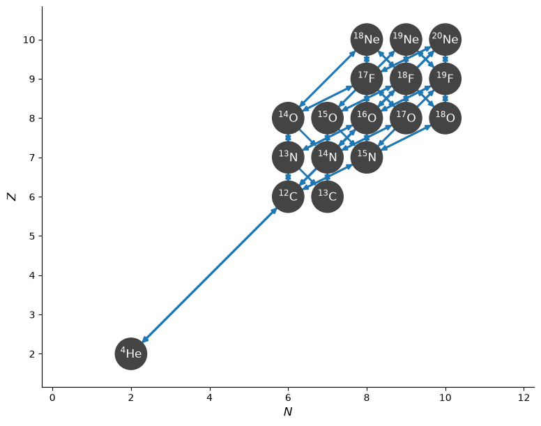
We can visualize the network and rates linking the nuclei

fig = net.plot()

pynucastro can write out the python code needed to evaluate the reaction rates

net.write_network("cno_integration_example.py")

/opt/hostedtoolcache/Python/3.14.7/x64/lib/python3.14/site-packages/pynucastro/rates/derived_rate.py:125: UserWarning: C12 partition function is not supported by tables: set log_pf = 0.0 by default
  warnings.warn(UserWarning(f'{nuc} partition function is not supported by tables: set log_pf = 0.0 by default'))
/opt/hostedtoolcache/Python/3.14.7/x64/lib/python3.14/site-packages/pynucastro/rates/derived_rate.py:125: UserWarning: N13 partition function is not supported by tables: set log_pf = 0.0 by default
  warnings.warn(UserWarning(f'{nuc} partition function is not supported by tables: set log_pf = 0.0 by default'))
/opt/hostedtoolcache/Python/3.14.7/x64/lib/python3.14/site-packages/pynucastro/rates/derived_rate.py:125: UserWarning: C13 partition function is not supported by tables: set log_pf = 0.0 by default
  warnings.warn(UserWarning(f'{nuc} partition function is not supported by tables: set log_pf = 0.0 by default'))
/opt/hostedtoolcache/Python/3.14.7/x64/lib/python3.14/site-packages/pynucastro/rates/derived_rate.py:125: UserWarning: N14 partition function is not supported by tables: set log_pf = 0.0 by default
  warnings.warn(UserWarning(f'{nuc} partition function is not supported by tables: set log_pf = 0.0 by default'))
/opt/hostedtoolcache/Python/3.14.7/x64/lib/python3.14/site-packages/pynucastro/rates/derived_rate.py:125: UserWarning: N15 partition function is not supported by tables: set log_pf = 0.0 by default
  warnings.warn(UserWarning(f'{nuc} partition function is not supported by tables: set log_pf = 0.0 by default'))

Now we can import the network that was just created

import cno_integration_example as cno

Structure of the ODE system

import inspect

print(inspect.getsource(cno.rhs_eq))

@numba.njit()
def rhs_eq(t, Y, rho, T, screen_func):

    rate_eval = do_rate_eval(t, Y, rho, T, screen_func)
    return ydot_eq(Y, rho, rate_eval)

Note

The forward and reverse rates are included for each link, and these are explicitly paired together to help with equilibrium.

Integrating with SciPy

We’ll use the BDF solver from SciPy solve_ivp method

from scipy.integrate import solve_ivp

Now we’ll set the thermodynamic conditions. We initialize mass fractions and then convert to molar fractions, since that’s what the RHS uses

rho = 150
T = 1.5e7

X0 = np.zeros(cno.nnuc)
X0[cno.jp] = 0.7
X0[cno.jhe4] = 0.28
X0[cno.jc12] = 0.02

Y0 = X0/cno.A

Notice that there are 2 separate tolerances–a relative and an absolute tolerance.

tmax = 1.e20

sol = solve_ivp(cno.rhs, [0, tmax], Y0, method="BDF",
                dense_output=True, args=(rho, T), rtol=1.e-6, atol=1.e-8)

sol.success

True

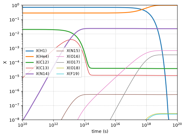
Now we can plot the mass fractions.

fig = plt.figure()
ax = fig.add_subplot(111)

for n in range(cno.nnuc):
    lw = 1
    max_X = (sol.y[n, :] * cno.A[n]).max()
    if max_X > 1.e-2:
        lw = 2
    if max_X > 1.e-8:
        ax.loglog(sol.t, sol.y[n, :] * cno.A[n],
                  lw=lw, label=f"X({cno.names[n].capitalize()})")

ax.set_xlabel("time (s)")
ax.set_ylabel("X")

ax.set_xlim(1.e10, 1.e20)
ax.set_ylim(1.e-8, 1.0)
ax.legend(fontsize="small", ncol=2)
ax.grid(ls=":")

try it…

What happens if we loosen the tolerances?