Lab 1 model profiles#
We’ll take a sneak peak at the profiles of the star from lab 1 at the start and end of the evolution.
You can download these as lab1/profile1.data and lab1/profile2.data.
import mesa_reader as mr
import matplotlib.pyplot as plt
import numpy as np
model1 = mr.MesaData("lab1/profile1.data")
model2 = mr.MesaData("lab1/profile2.data")
r1 = 10.0**model1.logR
m1 = model1.mass
rho1 = 10.0**model1.logRho
T1 = 10.0**model1.logT
r2 = 10.0**model2.logR
m2 = model2.mass
rho2 = 10.0**model2.logRho
T2 = 10.0**model2.logT
Here’s both models (dotted is the initial)
fig, ax = plt.subplots()
ax.loglog(r2, rho2, color="C0", label="density")
ax.loglog(r1, rho1, color="C0", ls=":")
ax.loglog(r2, T2, color="C1", label="temperature")
ax.loglog(r1, T1, color="C1", ls=":")
ax.legend()
ax.set_xlabel("radius [cm]")
ax.set_ylim(10, 5.e10)
ax.grid(ls=":")
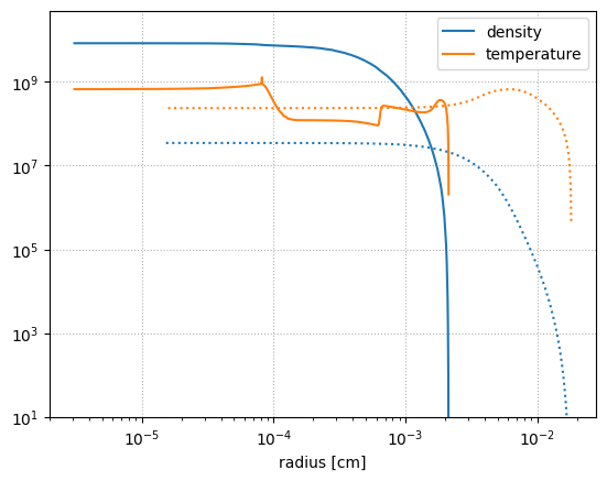
Notice that the final model is smaller in radius—white dwarfs shrink as they grow in mass.
EOS regimes#
Let’s see where these models lay in our EOS regimes diagram. The functions from that notebooks
are available in regimes.py.
import regimes
fig, ax = plt.subplots()
ax.loglog(rho1, T1, label="initial")
ax.loglog(rho2, T2, label="final")
ax.set_xlabel(r"$\rho$")
ax.set_ylabel("T")
ax.grid(ls=":")
ax.legend()

ax.set_xlim(1.e-5, 1.e11)
ax.set_ylim(1.e4, 1.e10)

rhos = np.logspace(-5, 11, 100)
ax.loglog(rhos, regimes.rad_ideal(rhos), color="0.5", ls="--")
ax.loglog(rhos, regimes.deg_ideal(rhos), color="0.5", ls="--")
ax.loglog(rhos, regimes.crystallization(rhos), color="0.5", ls="--")
[<matplotlib.lines.Line2D at 0x7f12e4fa0980>]
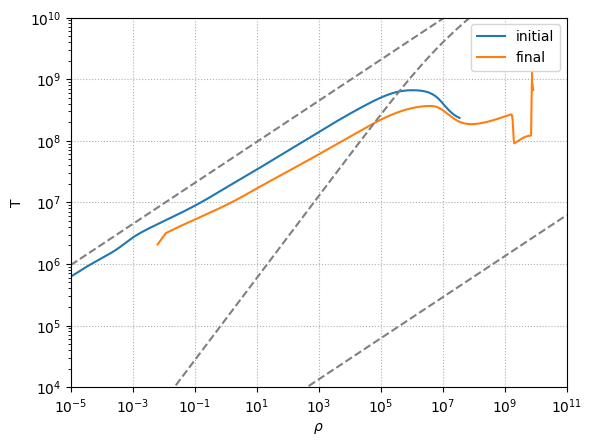
We see that our model is far from crystallizaton or radiation being important.