Degeneracy and White Dwarfs#
The Equation of State#
Inside of a star, once \(T \sim 10^4~\mathrm{K}\), atoms are fully ionized, so we treat ions and electrons separately. We also need to consider radiation pressure. We can write the total pressure in a star as:
Note
For stellar atmospheres, we are not in LTE (photons and matter don’t have the same temperature), photons are not trapped, and atoms may be only partially ionized.
We are only worrying about the stellar interior in this lab, so we can neglect these complications.
For stellar interiors we can describe these components as:
ions : these behave as an ideal gas (until we get to neutron stars), so we take:
\[P_\mathrm{ion} = \frac{\rho k_B T}{\mu_I m_u}\]where \(\mu_I\) is the mean molecular weight of the ions and \(m_u\) is the atomic mass unit.
radiation : photons are in equilibrium with matter and the mean free path is short compared to any scales we care about in the star, so we can treat them as a blackbody:
\[P_\gamma = \frac{1}{3} a T^4\]where \(a\) is the radiation constant.
electrons : these are tricky
at low densities / high temperatures, electrons behave as an ideal gas
at high densities / low temperatures, quantum mechanical effects become important. Because we are confining the electrons to a small volume, the Pauli exclusion principle comes into play, and says that the electrons need to take on high momentum. This gives rise to a quantum mechanical pressure we call degeneracy pressure.
Note
We usually include an additional contribution, Coulomb corrections, to the pressure. This accounts for the non-ideal nature of the ions (due to their electric charge) at high densities, and lowers the pressure.
Fermi-Dirac statistics#
We describe the statistics of particles through a distribution function:
For electrons, the distribution function is the Fermi-Dirac distribution.
where \(\mathcal{E}\) is the kinetic energy of the electron, \(T\) is the temperature, and \(\eta\) is the degeneracy parameter which is related to the chemical potential, \(\mu\), via:
Tip
See Understanding the chemical potential by Cook & Dickerson 1995 for a nice discussion on the chemical potential).
Note
At low density and high-temperature, electron-positron pairs can be produced, and we would need to consider the positron contribution to the EOS. For the conditions we will be looking at in the white dwarf interior, these will not be important.
Thermodynamic quantities#
To get the number density, we integrate over all momenta:
The pressure and specific internal energy, \(e\), are then found as:
Fermi energy#
We define Fermi energy, \(\mathcal{E}_F\), as:
and then
Degeneracy#
We can understand the behavior of the electrons in terms of \(\eta\):
\(-\eta \gg 1\) : the electrons behave as an ideal gas. In this case, the \(+1\) in the denominator of \(n(p)\) is insignificant and we get the Maxwell-Boltzmann distribution.
\(\eta \gg 1\) : the electrons are degenerate (Fermi energy is much greater than the thermal energy).
Transition to degeneracy#
Let’s look at the behavior of the distribution function. Consider:
let’s define
then we have
and for each choice of \(\eta\) we have a unique distribution.
We note that \(\xi/\eta = \mathcal{E}/\mathcal{E}_F\).
import numpy as np
import matplotlib.pyplot as plt
def F(xi, eta=100):
    return 1.0 / (np.exp(xi - eta) + 1)
Let’s look at the case of \(\eta > 1\)
fig, ax = plt.subplots()

# we'll work in terms of r = xi / eta
r = np.linspace(0, 4, 200)

for eta in [1, 2, 10, 20, 100]:
    ax.plot(r, F(eta * r, eta=eta), label=fr"$\eta = {eta}$")

ax.legend()
ax.set_ylabel("$F$")
ax.set_xlabel(r"$\mathcal{E}/\mathcal{E}_F$")
Text(0.5, 0, '$\\mathcal{E}/\\mathcal{E}_F$')
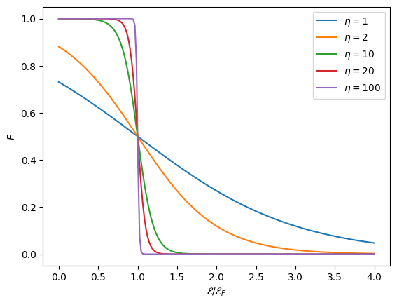
In the limit that \(T \rightarrow 0\) (complete degeneracy), then we have:
So the distribution function tends to a step-function when we are really degenerate and the most energetic electrons have a kinetic energy = Fermi energy.
Note
Conceptually:
At \(T = 0\), the Fermi energy is the energy of the highest occupied state in the distribution function.
Since electrons have a non-zero energy / momentum, even at \(T = 0\), there will be a pressure even in the limit \(T \rightarrow 0\)!
Even for non-zero \(T\), as long as \(\eta \gg 1\), we can still think of \(\mathcal{E}_F\) as being (roughly) the energy of the most energetic electrons.
We can think of \(\eta\) as (roughly) the ratio of the Fermi energy to the thermal energy
Fermi momentum#
We can alternately use the Fermi momentum, \(p_F\) to describe the location of the step. Two important limits are:
Zero-T limit#
For \(T \rightarrow 0\), the integral for number density is trivial:
where we switched to spherical coordinates in momentum space: \(d^3p \rightarrow 4\pi p^2 dp\).
Performing this integral, we get the Fermi momentum in terms of the number density of electrons:
Computing \(\eta\)#
For other values of \(\eta\), we have a problem:
We don’t know what the value of \(\eta\) is ahead of time. Instead, we typically know what the density of the star is, and we can find the number density of electrons as:
where \(Y_e\) is the electron fraction (typically around \(1/2\) for compositions heavier than hydrogen). This means that given \(\rho, T\), we can solve for \(\eta\).
The kinetic energy of a particle can be found from the relativisitic expression:
Note
This has the proper limit in the non-relativistic case, \(|p| \ll m_e c\):
Once we have \(\eta\), we can then find the pressure and energy of the gas.
Tip
We normally express these integrals in terms of energy. These integrals can be computed via pynucastro (see https://pynucastro.github.io/pynucastro/fermi-integrals.html)
A C++ code that computes these at very high precision is available at zingale/electron_positron_cxx
Finding the trend of \(\eta\) with \(\rho, T\)#
We will be interested in the Fermi energy / \(\eta\), so let’s look at the trend with density and temperature.
import pynucastro as pyna
eos = pyna.eos.ElectronEOS()
import numpy as np
comp = pyna.Composition(["o16", "ne20"])
comp.set_equal()
We’ll store \(\eta\) and \(P\) for a range of densities at a few different temperatures.
rhos = np.logspace(0, 9, 100)

etas = {}
ps = {}
for T in [1.e6, 1.e7, 1.e8]:
    etas[T] = []
    ps[T] = []
    for rho in rhos:
        # by default, this gives both the electron and
        # positron contributions.  We'll ignore the positrons
        ee, _ = eos.pe_state(rho, T, comp)
        etas[T].append(ee.eta)
        ps[T].append(ee.p)
Let’s visualize \(\eta\)
fig, ax = plt.subplots()

for T in etas:
    ax.plot(rhos, etas[T], label=f"T = {T:5.2g}")

ax.set_xlabel(r"$\rho$")
ax.set_ylabel(r"$\eta$")
ax.set_xscale("log")
ax.set_yscale("symlog", linthresh=1.e-2)
ax.legend()
ax.grid(ls=":")
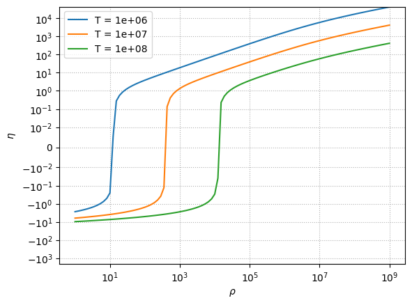
We’ll have \(\rho > 10^9~\mathrm{g~cm^{-3}}\) in the core of our white dwarf, so we will have a high \(\eta\).
Let’s redo this plot in terms of Fermi energy.
k = pyna.constants.constants.k_MeV

fig, ax = plt.subplots()

for T in etas:
    ax.plot(rhos, np.array(etas[T]) * k * T, label=f"T = {T:5.2g}")

ax.set_xlabel(r"$\rho$")
ax.set_ylabel(r"$\mathcal{E}_F$ (MeV)")
ax.set_xscale("log")
ax.set_yscale("symlog", linthresh=1.e-3)
ax.legend()
ax.grid(ls=":")
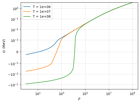
Important
We see that at high density, the Fermi energy is a few MeV. This is comparable to the binding energy / nucleon in a nucleus.
Pressure at zero-T#
At zero-temperature, the distribution function is a step function, and then integrals become straightforward.
The number density is just:
or, the Fermi momentum is:
For the pressure, we need \(v(p)\), which from mechanics is:
and taking \(T \rightarrow 0\), our pressure integral becomes:
Performing this integral, we find:
where \(x\) is the dimensionless Fermi momentum,
and using our Fermi momentum expression,
Note
The boundary between non-relativistic and relativistic is \(x \sim 1\)
We can take the limits of our \(P(x)\) expression, and putting back in \(x\) in terms of \(\rho\), we would find:
Exploring the transition to degeneracy#
We can compare the exact expression to this zero-T expression to see when the transition to degeneracy occurs.
m_u = pyna.constants.constants.m_u
h_planck = pyna.constants.constants.h
c = pyna.constants.constants.c_light
m_e = pyna.constants.constants.m_e
def p_zero_temp(rho, Ye=0.5):

    # find number density
    n_e = rho * Ye / m_u

    # find Fermi momentum
    x_F = (3 / (8 * np.pi))**(1/3) * (h_planck / (m_e * c)) * n_e**(1/3)

    P = (np.pi/3) * (m_e * c / h_planck)**3 * m_e * c**2 * (x_F * (2*x_F**2 - 3) *
                                                            np.sqrt(1 + x_F**2) + 3 *
                                                            np.arcsinh(x_F))
    return P
fig, ax = plt.subplots()

for T in ps:
    ax.loglog(rhos, ps[T], label=f"T = {T:5.2g}")

ax.loglog(rhos, p_zero_temp(rhos), linestyle=":", color="0.5", label="zero-T")

ax.set_xlabel(r"$\rho$")
ax.set_ylabel(r"$P$")
ax.grid(ls=":")
ax.legend()
<matplotlib.legend.Legend at 0x7f46cff87620>
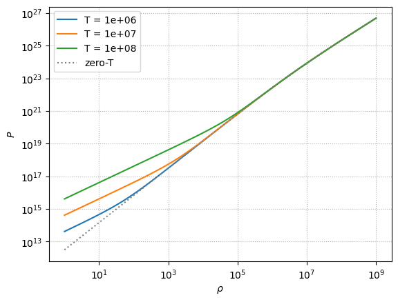
We see that at high density, the pressure matches the zero-T approximation well. At lower densities, the electrons break from the zero-T curve and act as an ideal gas.