Networks used in labs

In the labs, we build minimal networks with only a subset of the rates that can connect the nuclei.

We will focus on the \(A = 23\) and \(A = 25\) Urca pairs.

Why odd-mass numbers for Urca?

This was addressed in the seminal paper by Tsuruta & Cameron 1970:

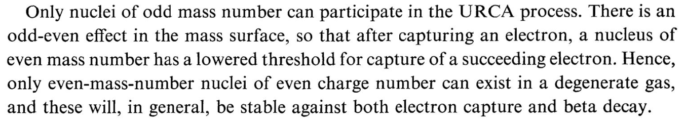
Their argument is that for even mass number, \(A\), nuclei with an even \(Z\) (proton number) and even \(N\) (neutron number) are the most stable. If a (\(Z\) even, \(N\) even) nucleus captures and electron, then we get (\(Z\) odd, \(N\) odd) and this is likely to very quickly capture another electron.

This breaks the pairing of electron-capture and \(\beta\)-decay for even \(A\) nuclei.

O+O rate

These nets all use an approximation to the O+O burning rate

import pynucastro as pyna
from pynucastro.rates.aprox_family_rates import make_CO_approx_rates

rl = pyna.ReacLibLibrary()
o_rates = make_CO_approx_rates(rl.get_rates(), "O")
o_rates

[O16 + O16 ⟶ S32 + 𝛾,
 S32 ⟶ O16 + O16,
 O16 + O16 ⟶ Si28 + He4,
 Si28 + He4 ⟶ O16 + O16,
 Si28 + He4 ⟶ S32 + 𝛾,
 S32 ⟶ Si28 + He4]

net = pyna.RateCollection(rates=o_rates)
fig = net.plot(rotated=True, curved_edges=True)

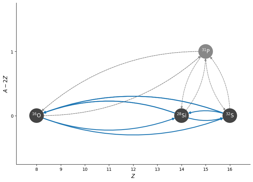
We see that we can go from \({}^{16}\mathrm{O}\) to \({}^{28}\mathrm{Si}\) either directly, or through \({}^{31}\mathrm{P}\). We’ll use an approximate rate that represents both of these paths

r1616 = net.get_rate_by_name("o16(o16,he4)si28")
r1616

O16 + O16 ⟶ Si28 + He4

type(r1616)

pynucastro.rates.approximate_rates.ApproximateRate

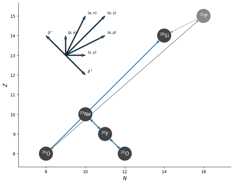
Lab 1

We’ll use the tabular rates from Suzuki

sl = pyna.SuzukiLibrary()

rate_names = ["ne20(,)f20",
              "f20(,)ne20",
              "f20(,)o20",
              "o20(,)f20"]
rates = sl.get_rate_by_name(rate_names)

net = pyna.RateCollection(rates=[r1616]+rates)

fig = net.plot(legend_coord=(13, 9))

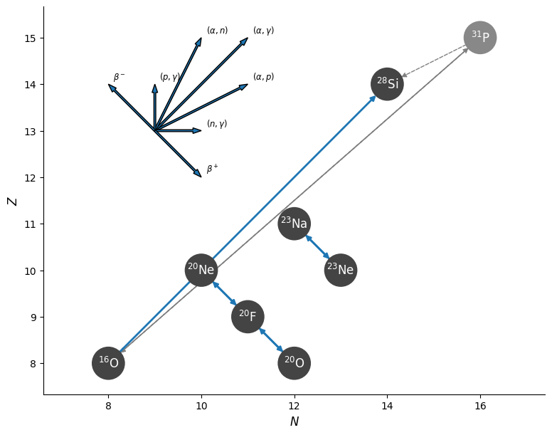
Lab 2

first Urca pair

rate_names += ["na23(,)ne23",
               "ne23(,)na23"]
rates = sl.get_rate_by_name(rate_names)

net = pyna.RateCollection(rates=[r1616]+rates)
fig = net.plot(legend_coord=(13, 9))

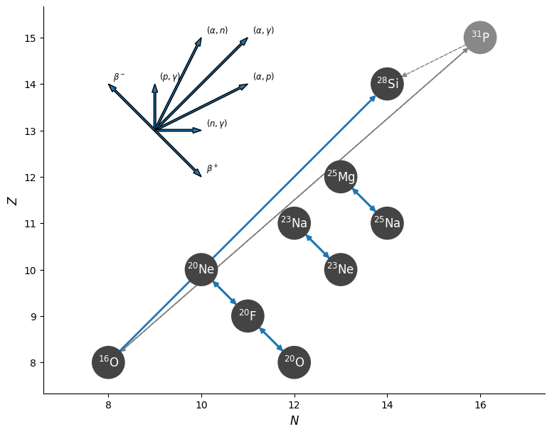
second Urca pair

rate_names += ["mg25(,)na25",
               "na25(,)mg25"]
rates = sl.get_rate_by_name(rate_names)

net = pyna.RateCollection(rates=[r1616]+rates)
fig = net.plot(legend_coord=(13, 9))

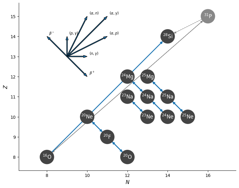
Lab 3

We add a second \(A=25\) urca pair and some \(A = 24\) rates

rate_names += ["mg24(,)na24",
               "na24(,)mg24",
               "na24(,)ne24",
               "ne24(,)na24",
               "na25(,)ne25",
               "ne25(,)na25"]
rates = sl.get_rate_by_name(rate_names)

net = pyna.RateCollection(rates=[r1616]+rates)
fig = net.plot(legend_coord=(13, 9))