Thermodynamics and the Maxwell-Boltzmann distribution

Here we use SymPy to learn a bit about ideal gases

from sympy import init_session
init_session(use_latex="mathjax")
%matplotlib inline

IPython console for SymPy 1.13.3 (Python 3.11.10-64-bit) (ground types: python)

These commands were executed:
>>> from sympy import *
>>> x, y, z, t = symbols('x y z t')
>>> k, m, n = symbols('k m n', integer=True)
>>> f, g, h = symbols('f g h', cls=Function)
>>> init_printing()

Documentation can be found at https://docs.sympy.org/1.13.3/

Note: we need to tell SymPy that some of these quantities are real and positive so it is able to do the integrals without worrying about complex numbers

ni, m, k, T = symbols("n_I m k_B T", real=True, positive=True)
p, v = symbols("p v", real=True)
n = symbols("n")

Let’s write the Maxwell-Boltzmann distribution, already transformed into spherical coordinates:

\[n(p) d^3 p \rightarrow 4\pi p^2 n(p) dp\]

our n here includes the \(4\pi p^2\)

n = 4*pi* p**2 * ni / (2 * pi * m * k *T)**Rational(3,2) * exp(-p**2/(2*m*k*T))
n

\[\displaystyle \frac{\sqrt{2} n_{I} p^{2} e^{- \frac{p^{2}}{2 T k_{B} m}}}{\sqrt{\pi} T^{\frac{3}{2}} k_{B}^{\frac{3}{2}} m^{\frac{3}{2}}}\]

average velocity

We want to compute the average velocity:

\[\langle v \rangle = \frac{1}{n_I} \int_{-\infty}^{\infty} n(v)v d^3 v\]

We’ll express \(v = p / m\) and work in terms of momentum

\[\langle v \rangle = \frac{1}{m n_I} \int_{-\infty}^{\infty} n(p) p d^3 p\]

now switching to spherical coordinates in momentum space:

\[\langle v \rangle = \frac{1}{m n_I} \int_{0}^{\infty} 4 \pi n(p) p^3 dp\]

vavg = (1/ni) * integrate(n * p / m, (p, 0, oo))
vavg

\[\displaystyle \frac{2 \sqrt{2} \sqrt{T} \sqrt{k_{B}}}{\sqrt{\pi} \sqrt{m}}\]

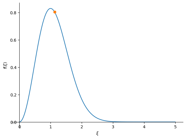
Notice that this value is greater than the most likely velocity (where the peak of the M-B) distribution is. This is because there is a long tail to high velocities. We can see this via a plot

xi = symbols("xi")

We’ll define a dimensionless momentum to allow us to plot this:

\[\xi = \frac{p}{\sqrt{2mkT}}\]

Then

\[n(p)dp \rightarrow n(\xi) d\xi\]

with \(n(xi) d\xi\) as

n_dxi = n.subs(p, sqrt(2*m*k*T)*xi)/ni * sqrt(2*m*k*T)

and our average velocity is then:

xi_avg = m * vavg / sqrt(2*m*k*T)
xi_avg

\[\displaystyle \frac{2}{\sqrt{\pi}}\]

fig = plot(n_dxi, (xi, 0, 5),
           markers=[{'args': [[xi_avg], [n_dxi.subs(xi, xi_avg)], "o"]}])

Here we see that the average velocity is slightly larger than the most probably velocity (the location of the peak).