Homework #1 stellar model

I’m using SymPy, the symbolic math library for python, to do the algebra here. The next 2 cells load SymPy for interactive work and define the variables we are going to use (and treat as math symbols)

from sympy import init_session
init_session(use_latex="mathjax")
%matplotlib inline

IPython console for SymPy 1.13.3 (Python 3.11.10-64-bit) (ground types: python)

These commands were executed:
>>> from sympy import *
>>> x, y, z, t = symbols('x y z t')
>>> k, m, n = symbols('k m n', integer=True)
>>> f, g, h = symbols('f g h', cls=Function)
>>> init_printing()

Documentation can be found at https://docs.sympy.org/1.13.3/

rho = symbols('rho', cls=Function)
qc = symbols('q_c')
pc = symbols('p_c')
G = symbols('G')
Mstar, Rstar = symbols(r'M_\star R_\star')
r = symbols('r')
xi = symbols('xi')
beta = symbols('beta')

Consider a mass profile in a star:

\[m(r) = 4\pi R^3 \beta \left [ \frac{1}{9} \left (\frac{r}{R} \right )^3 - \frac{1}{18} \left ( \frac{r}{R} \right)^6 \right ]\]

where \(\beta\) is a constant

a. density profile

What is the density profile, \(\rho(r)\), that gives rise to this mass?

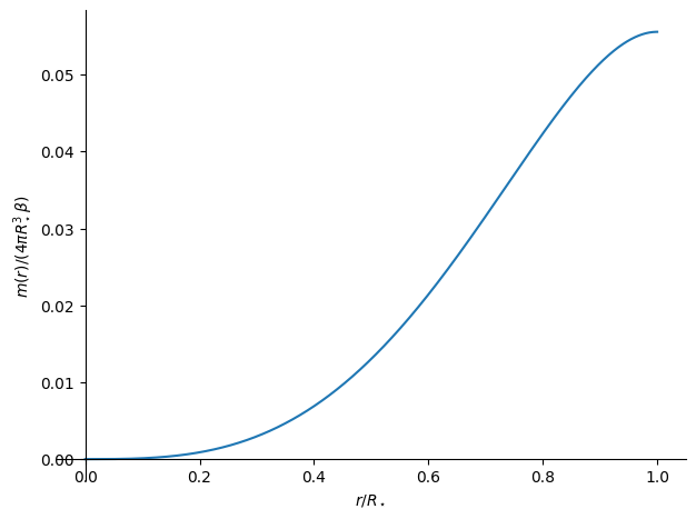
First let’s plot the function \(m(r)\)

m = 4*pi*Rstar**3*beta*(Rational(1, 9) * (r/Rstar)**3 - Rational(1, 18) * (r/Rstar)**6)
m

\[\displaystyle 4 \pi R_{\star}^{3} \beta \left(\frac{r^{3}}{9 R_{\star}^{3}} - \frac{r^{6}}{18 R_{\star}^{6}}\right)\]

To make the plot we need to make it dimensionless, so we’ll define \(\xi = r/ R\).

z = (m/(4*pi*Rstar**3*beta)).subs(r, xi*Rstar)
plot(z, (xi, 0, 1), xlabel=r"$r/R_\star$", ylabel=r"$m(r)/(4\pi R_\star^3\beta)$")

<sympy.plotting.backends.matplotlibbackend.matplotlib.MatplotlibBackend at 0x7fb3dc62f810>

Now we get the density as

(4)\[\begin{equation} \rho = \frac{1}{4\pi r^2} \frac{dm}{dr} \end{equation}\]

rho = m.diff(r, 1)/(4*pi*r**2)
rho = simplify(rho)
rho

\[\displaystyle \frac{\beta \left(R_{\star}^{3} - r^{3}\right)}{3 R_{\star}^{3}}\]

b. central density

What is \(\beta\) in terms of the central density?

The central density is just \(\rho(0)\)

rhoc = rho.subs(r, 0)
rhoc

\[\displaystyle \frac{\beta}{3}\]

So \(\beta = 3 \rho_c\). We can rewrite the density in terms of \(\rho_c\) now

rhoc = symbols("rho_c")
rho = simplify(rho.subs(beta, 3*rhoc))
rho

\[\displaystyle \rho_{c} - \frac{r^{3} \rho_{c}}{R_{\star}^{3}}\]

We can also rewrite the mass, \(m(r)\), in terms of \(\rho_c\):

m = simplify(m.subs(beta, 3*rhoc))
m

\[\displaystyle \frac{2 \pi r^{3} \rho_{c} \left(2 R_{\star}^{3} - r^{3}\right)}{3 R_{\star}^{3}}\]

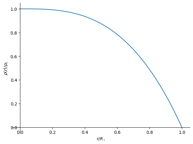
Notice that the density vanishes at \(r = R_\star\). Now let’s plot this.

z = simplify((rho/rhoc).subs(r, xi*Rstar))
plot(z, (xi, 0, 1), xlabel=r"$r/R_\star$", ylabel=r"$\rho(r)/\rho_c$")

<sympy.plotting.backends.matplotlibbackend.matplotlib.MatplotlibBackend at 0x7fb394ac5150>

c. ratio of central to average

What is the ratio of the central density to the average density, \(\rho_c / \bar{\rho}\)?

The average density is just the total mass divided by the volume of the star. First we get the total mass, \(M_\star = m(R_\star)\)

Mstar = m.subs(r, Rstar)
Mstar

\[\displaystyle \frac{2 \pi R_{\star}^{3} \rho_{c}}{3}\]

and now we compute

(5)\[\begin{equation} \bar{\rho} = \frac{M_\star}{(4/3) \pi R_\star^3} \end{equation}\]

rhobar = symbols(r"\bar{\rho}")
rhobar = Mstar / (Rational(4,3)*pi*Rstar**3)
rhobar

\[\displaystyle \frac{\rho_{c}}{2}\]

So \(\bar{\rho} = \rho_c/2\) and the ratio of \(\rho_c/\bar{\rho}\) is 2.

Alternately, we can do a volume-weighted average of \(\rho(r)\):

(6)\[\begin{equation} \bar{\rho} = \frac{1}{V} \int_0^R 4\pi r^2 \rho(r) dr \end{equation}\]

integrate(4*pi*r**2*rho, (r, 0, Rstar)) / (Rational(4,3)*pi*Rstar**3)

\[\displaystyle \frac{\rho_{c}}{2}\]

d. central pressure

What is the central pressure of the star for this mass distribution?

Now we can integrate HSE. We will do this as

\[p = p_c + \int_0^{R_\star} \frac{-Gm(r)}{r^2} \rho dr\]

Here I’ve written the integral in terms of \(r\). We’ll substitute in our expressions for \(m(r)\) and \(\rho(r)\) in the integrand.

pc = symbols("p_c")
p = pc + integrate(-G*m/r**2*rho, (r, 0, Rstar))
p

\[\displaystyle - \frac{7 \pi G R_{\star}^{2} \rho_{c}^{2}}{20} + p_{c}\]

This was the integral to the surface, so this result is the surface pressure, but we know that \(p(R_\star) = 0\), so we can enforce that here to find \(p_c\)

pc = solve(Eq(p, 0), pc)[0]
pc

\[\displaystyle \frac{7 \pi G R_{\star}^{2} \rho_{c}^{2}}{20}\]

This is \(p_c\) in terms of \(\rho_c\), but we can substitute in \(\rho_c = 2 \bar{\rho}\) to find the central pressure in terms of \(M_\star\) and \(R_\star\). (Note to make the code use \(M_\star\) and not its equivalent in terms of \(\rho_c\) found above, I am defining a new symbol \(M\) here that will represent the total mass of the star.)

M = symbols("M")
pc.subs(rhoc, 2*M/(Rational(4,3)*pi*Rstar**3))

\[\displaystyle \frac{63 G M^{2}}{80 \pi R_{\star}^{4}}\]

From this expression, we see that \(f = 63/(80\pi)\).

e. gravitational potential

What is the total gravitational potential energy, \(\Omega\), of the star?

We integrate

\[\Omega = -\int_0^{M_\star} \frac{Gm(r)}{r} dm = -\int_0^{R_\star} \frac{G m(r)}{r} 4\pi r^2 \rho dr\]

To do this, we use our expression for \(m(r)\) and \(\rho(r)\)

Omega = symbols("Omega")
Omega = integrate(-G*m*4*pi*r*rho, (r, 0, Rstar))

Omega

\[\displaystyle - \frac{17 \pi^{2} G R_{\star}^{5} \rho_{c}^{2}}{55}\]

We can rewrite this in terms of mass, by using \(\rho_c = 2 \bar{\rho}\) that we found for this model above

Omega = Omega.subs(rhoc, 2*M/(Rational(4,3)*pi*Rstar**3))
Omega

\[\displaystyle - \frac{153 G M^{2}}{220 R_{\star}}\]

So this shows that \(\alpha = 153/220\).