
Implicit Methods and Nonlinear Systems
Contents
import numpy as np
import matplotlib.pyplot as plt
import matplotlib as mpl
mpl.rcParams['figure.dpi'] = 100
mpl.rcParams['figure.figsize'] = (10, 8)
Implicit Methods and Nonlinear Systems#
Nonlinear system#
Consider the following nonlinear system:
The Jacobian is:
(this example comes from the VODE documentation)
We’ll use the intiial conditions
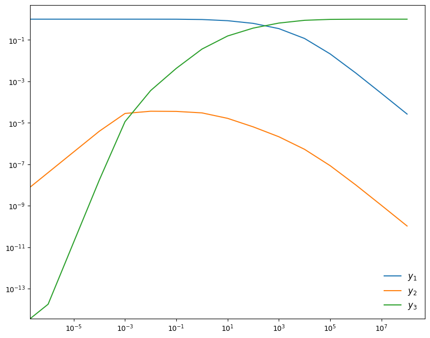
This system has the longterm behavior that:
Although \(y_2\) is initially 0, it will build up quickly and feed the creation of \(y_3\).
Linearization#
Let’s write our system as:
We will discretize this as:
We will linearize the righthand side. We’ll start with an initial guess for the new-time solution, \({\bf y}_0^{n+1}\), and seek a correction, \(\Delta {\bf y}_0\) such that:
Now we insert this in \({\bf f}\) and Taylor expand:
Our linearized system becomes:
or in terms of the correction:
This is a linear system that we can solve. The basic idea will be:
Apply the correction
Check for convergence: \(\| \Delta {\bf y} \| < \epsilon \| {\bf y}^n \|\)
Iterate, finding the next correction until we converge
Backward Euler Implementation#
First we need functions for the righthand side and Jacobian
def rhs(t, Y):
    """ RHS of the system -- using 0-based indexing """
    y1 = Y[0]
    y2 = Y[1]
    y3 = Y[2]

    dy1dt = -0.04*y1 + 1.e4*y2*y3
    dy2dt =  0.04*y1 - 1.e4*y2*y3 - 3.e7*y2**2
    dy3dt =                         3.e7*y2**2

    return np.array([dy1dt, dy2dt, dy3dt])

def jac(t, Y):
    """ J_{i,j} = df_i/dy_j """

    y1 = Y[0]
    y2 = Y[1]
    y3 = Y[2]

    df1dy1 = -0.04
    df1dy2 = 1.e4*y3
    df1dy3 = 1.e4*y2

    df2dy1 = 0.04
    df2dy2 = -1.e4*y3 - 6.e7*y2
    df2dy3 = -1.e4*y2

    df3dy1 = 0.0
    df3dy2 = 6.e7*y2
    df3dy3 = 0.0

    return np.array([ [ df1dy1, df1dy2, df1dy3 ],
                      [ df2dy1, df2dy2, df2dy3 ],
                      [ df3dy1, df3dy2, df3dy3 ] ])
Next we’ll write the main driver. This integrates from [t, tmax] using a timestep dt_init. We specify a tolerance for the convergence of the nonlinear system solve for each step.
SMALL = 1.e-100

def backwards_euler(t, tmax, dt_init, y_init, rhs, jac,
                    tol=1.e-6, max_iter=100):
    """solve the system dy/dt = f(y), where f(y) is provided by the
    routine rhs(), and the Jacobian is provided by the routine jac().

      t : the current time
      tmax : the ending time of integration
      dt_init : initial timestep
      y_init : the initial conditions

    """

    time = t
    dt = dt_init

    # starting point of integration of each step
    y_n = np.zeros_like(y_init)
    y_n[:] = y_init[:]

    y_new = np.zeros_like(y_init)

    while time < tmax:

        converged = False

        # we want to solve for the updated y.  Set an initial guess to
        # the current solution.
        y_new[:] = y_n[:]

        err = 1.e30
        niter = 0

        neq = len(y_init)

        while err > tol and niter < max_iter:

            # construct the matrix A = I - dt J
            A = np.eye(neq) - dt * jac(time, y_n)

            # construct the RHS
            b = y_n - y_new + dt * rhs(time, y_new)

            # solve the linear system A dy = b
            dy = np.linalg.solve(A, b)

            # correct our guess
            y_new += dy

            # check for convergence
            err = np.linalg.norm(dy) / np.linalg.norm(y_new) #max(abs(y_new) + SMALL)
            niter += 1

        if time + dt > tmax:
            dt = tmax - time

        y_n[:] = y_new[:]
        time += dt

    return y_n
We’ll follow the example from the VODE documentation and integrate in several chunks. We’ll evolve from \(t = 0\) stopping at \(t = 10^{-6}, 10^{-5}, \ldots 10^8\). Each call to the integrator will begin with the time from the previous integration, and we’ll always set \(\tau\) to have ~10 steps per interval.
y_init = np.array([1.0, 0.0, 0.0])

# like the vode driver, we will do the integration in a bunch of
# pieces, increasing the stopping time by 10x each run
tends = np.logspace(-6, 8, 15)

time = 0.0
y_old = y_init.copy()

ys = []
for y in y_init:
    ys.append([y])

ts = [time]

total_be_solves = 0

for tmax in tends:

    y_new = backwards_euler(time, tmax, tmax/10, y_old, rhs, jac)

    time = tmax
    ts.append(time)
    for n, y in enumerate(y_new):
        ys[n].append(y)

    y_old[:] = y_new[:]
Now we can plot the 3 species
fig = plt.figure()
ax = fig.add_subplot(111)

for n, y in enumerate(ys):
    ax.plot(ts, y, label=rf"$y_{n+1}$")

ax.legend(frameon=False, fontsize="large")
ax.set_xscale("log")
ax.set_yscale("log")
Comparison of Methods#
from scipy.integrate import solve_ivp
Now we can try integrating this system using any of the methods built into SciPy https://docs.scipy.org/doc/scipy/reference/generated/scipy.integrate.solve_ivp.html
We are successful if we try BDF, but we fail if we try the RK45 method. This is an emperical demonstration that this problem is stiff.
sol = solve_ivp(rhs, [0, 1.e8], [1, 0, 0], method="BDF", dense_output=True)
print(sol)
  message: The solver successfully reached the end of the integration interval.
  success: True
   status: 0
        t: [ 0.000e+00  3.196e-05 ...  9.399e+07  1.000e+08]
        y: [[ 1.000e+00  1.000e+00 ...  2.209e-05  2.075e-05]
            [ 0.000e+00  1.277e-06 ...  8.836e-11  8.300e-11]
            [ 0.000e+00  1.320e-09 ...  1.000e+00  1.000e+00]]
      sol: <scipy.integrate._ivp.common.OdeSolution object at 0x7fb3a2ad7490>
 t_events: None
 y_events: None
     nfev: 443
     njev: 12
      nlu: 57