import numpy as np
import matplotlib.pyplot as plt

from scipy import special

Exercises

1. Second derivative

We can compute a second derivative in the same fashion as we did for the first derivative—starting with the Taylor expansion about \(x_i\) and solving for the second derivative approximation at \(i\).

Work out the Taylor expansion and compute the second derivative of \(f(x) = \sin(x)\) on a grid of 10 points from \([0, \pi]\) at the point x[3].

Consider the two Taylor expansions from before:

\[f_{i+1} = f_i + \Delta x \left .\frac{df}{dx} \right |_i + \frac{1}{2} \Delta x^2 \left . \frac{d^2f}{dx^2} \right |_i + \frac{1}{6} \Delta x^3 \left . \frac{d^3f}{dx^3} \right |_i + \mathcal{O}(\Delta x^4)\]

and

\[f_{i-1} = f_i - \Delta x \left .\frac{df}{dx} \right |_i + \frac{1}{2} \Delta x^2 \left . \frac{d^2f}{dx^2} \right |_i - \frac{1}{6} \Delta x^3 \left . \frac{d^3f}{dx^3} \right |_i + \mathcal{O}(\Delta x^4)\]

Now add them, instead of subtracting them:

\[f_{i+1} + f_{i-1} = 2 f_i + \Delta x^2 \left . \frac{d^2f}{dx^2} \right |_i + \mathcal{O}(\Delta x^4)\]

and solve for the second derivative

\[\left . \frac{d^2f}{dx^2} \right |_i = \frac{f_{i+1} - 2 f_i + f_{i-1}}{\Delta x^2} + \mathcal{O}(\Delta x^2)\]

x = np.linspace(0, np.pi, 20, endpoint=False)

def f(x):
    return np.sin(x)

def second_deriv(x, idx):
    dx = x[idx] - x[idx-1]
    return (f(x[idx+1]) - 2*f(x[idx]) + f(x[idx-1]))/dx**2

print(second_deriv(x, 6), -np.sin(x[6]))

-0.8073548874068714 -0.8090169943749475

2. Integrating to infinity

If our integration limits extend to infinity, we cannot divide the infinite domain into slabs and compute the area under them directly. Instead we transform the integral. Consider the gamma function:

\[ \Gamma(a) = \int_0^\infty x^{a-1} e^{-x} dx \]

The integrand has a maximum at \(x = a-1\).

To evaluate this numerically, consider a variable transformation of the form:

\[ z = \frac{x}{c + x} \]

with \(c = a - 1\), corresponding to the maximum of the integrand.

With this change of variables, we map \(x \in [0, \infty)\) to \(z \in [0, 1]\). (Note: this transformation should only be used for \(a > 1\)).

Reexpress the integral in terms of \(z\) and do the numerical integration. Compare to the true value of \(\Gamma(a)\) for a few values of \(a > 1\).

(based on Newman)

Our change of variables is:

\[ x = c \frac{z}{1-z}\]

and

\[dx = \frac{cdz}{(1-z)^2}\]

so our integral:

\[ \Gamma(a) = \int_0^\infty \phi(x) dx\]

becomes

\[\Gamma(a) = c \int_0^1 \phi\left (c \frac{z}{1-z}\right ) (1 - z)^{-2} dz\]

Our code is:

# this is a safety factor to prevent NaNs
SMALL = 1.e-20

def integrand(x, a):
    """ the original integrand of our integral"""
    
    # note for a != 1, the integrand is 0 if x == 0

    return np.where(x > 0.0,
                    x**(a-1)*np.exp(-x), 0.0)

def zv(x, a):
    """ transform the variable x -> z """
    c = a - 1.0
    return x/(c + x) 

def xv(z, a):
    """ transform back from z -> x """
    c = a - 1.0
    return c*z/(1.0 - z + SMALL)

def gamma_integral(a, npts):
    """ integrate the gamma function """
    
    z = np.linspace(0.0, 1.0, npts)

    # do the integral via the trapezoid rule.  We will integrate
    # over z = [0, 1].  Our integral, with our change of coords
    # is 
    #
    # I = c int_0^1 f( (z/(1-z)) ) dz/(1-z)^2
    
    I = 0.0
    f = integrand(xv(z, a), a)
    c = a - 1.0

    for n in range(1, npts):
        I += 0.5*(z[n] - z[n-1])*(f[n]/(1.0 - z[n] + SMALL)**2 + 
                                  f[n-1]/(1.0 - z[n-1] + SMALL)**2)
    I *= c

    return I

a = 1.5
N = 200
I = gamma_integral(a, N)
print(I)

0.8862007113724983

We can compare to the value from scipy

special.gamma(a)

0.8862269254527579

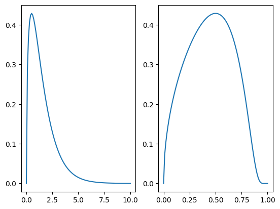
Note: this change of variables is designed to put the peak of the integrand at \(z = 1/2\). We can see that by plotting.

a = 1.5

fig = plt.figure()
ax = fig.add_subplot(121)

x = np.linspace(0, 10, 100)
ax.plot(x, integrand(x, a))
#ax.set_yscale("log")

ax = fig.add_subplot(122)
z = np.linspace(0, 1, 100)
ax.plot(z, integrand(xv(z, a), a))
#ax.set_yscale("log")

[<matplotlib.lines.Line2D at 0x7fcd07d3c580>]